msrDynamics

Documentation Under Construction

msrDynamics is an object-oriented API for constructing and solving reduced order thermal hydraulic systems, written with emulation of Simulink-style solvers for molten salt reactor (MSR) systems in mind (e.g. Singh et al), but can be extended to other fission and/or thermal hydraulic systems. The goal of this package is to streamline the implementation of such nodal models for more complex systems, where direct handling of the equations can become cumbersome.

Theory & Background

The API is designed for building nodal systems where variables representing system components or masses are aggregated into nodes with associated properties, and which only interact with other nodes through these properties. The nodes therefore, are essentially representations of the state variables of a first-order system of differential equations, suitable for a numerical solver.

A first-order system of ODEs (ordinary differential equations) takes the form

\[\dot{y} = f(t, y, \ldots)\]

For MSRs and other thermal hydraulic systems, the dynamics of the state at a given time, \(\dot{y(t)}\), depend on the state at time \(t\), \(y(t)\), but may also depend on the state at some previous time \(y(t-\tau)\) where \(\tau = (\tau_1, \tau_2, ...)\) are the respective delay times of the relevant state variables. The system to be solved is therefore a delay differential equation of the form

\[\dot{y} = f(t, y(t), y(t-\tau_1), y(t-\tau_2), \ldots)\]

msrDynamics essentially provides tools to construct symbolic expressions representing a system of this form, which are then passed to JiTCDDE as the backend solver. JiTCDDE integrates adaptively using a Bogacki-Shampine pair. The state and derivative of the system or stored at each integration step, which allows for past states to be evaluated using piece-wise cubic hermite interpolation. This is the DDE integration method proposed by Shampine and Thompson [ST01].

Modeling Approach

The model essentially describes heat flow through the component masses, aggregating all spatial considerations into zero-dimensional (spatial) relationships governed by constant coefficients. Listed below is some relevant literature on this approach and its applications:

The figure below shows an MSR core, modeled after that of the Aircraft Reactor Experiment (ARE). Each node is represented by its mass and thermophysical properties.

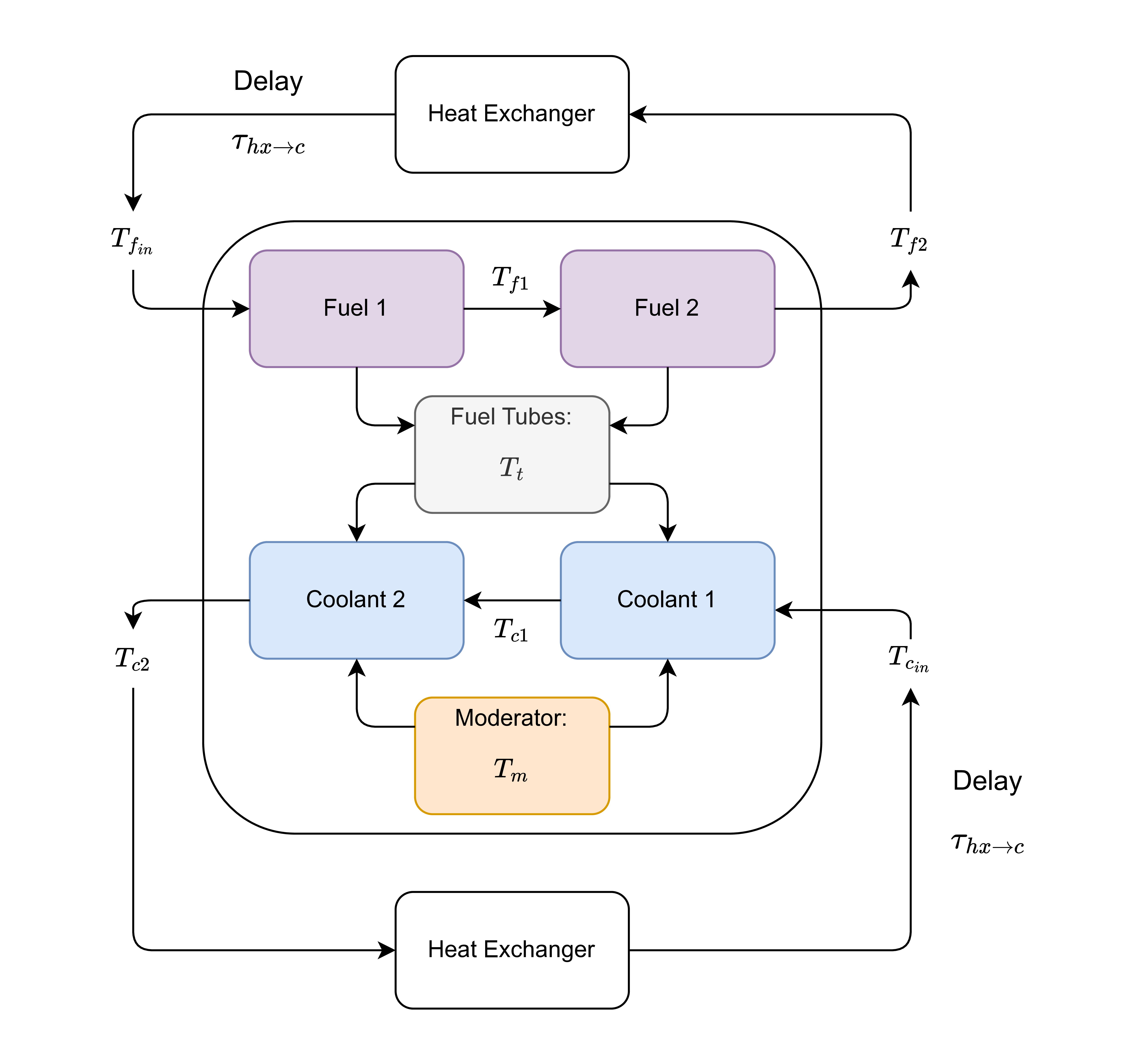
The ARE core consisted of NaF-ZrF4-UF4 fuel which flowed through inconel tubes making several passes through BeO moderator blocks. A liquid sodium coolant flowed in the opposite direction, in direct contact with the moderator blocks and fuel tubes. The arrows in the figure above represent the heat flows considered in the model. For example, there is advective heat flow between Fuel 1 and Fuel 2. Both are in contact with the tubes. As such there is convective heat exchange between the fuel and the fuel tubes.

Usage & API Description

The Node() object includes helper functions to define symbolic expressions representing convective and advective heat transfer, as well as generation from point-kinetics. User-defined dynamics are supported as well. The ARE core (shown above) can be modelled as follows

from msrDynamics import Node, System

# instantiate system object
ARE = System()

# mass, kg
m_fuel_core      = 100.0
m_coolant_core   = 100.0
m_tubes_core     = 100.0
m_moderator_core = 350.0

# specific heat capacity MW/°K
scp_fuel      = 2.0e-3
scp_coolant   = 4.0e-3
scp_moderator = 2.0e-3
scp_tubes     = 0.5e-3

# flow rate, kg/s
W_fuel    = 100.0
W_coolant = 50.0

# convection heat transfer coefficients, MW/°K
hA_fuel_tubes = 0.1
hA_coolant_tubes = 0.4

# delays
tau_c = 12.0
tau_l = 16.0

# inlet temperatures
T_f_in = 650
T_c_in = 500

# power in MW & fraction of power generated in fuel nodes
P = 2.0
P_f_1 = 0.5*P
P_f_2 = 0.5*P

# neutronics parameters
Lam = 1.32e-04                                                                  # mean generation time (openmc ifp branch)
lam = np.array([1.240E-02, 3.05E-02, 1.11E-01, 3.01E-01, 1.140E+00, 3.014E+00]) # precursor decay constants
beta = (np.array([0.000223, 0.001457, 0.001307, 0.002628, 0.000766, 0.00023]))  # delayed precursor yield
beta_t = np.sum(beta)                                                           # total delayed neutron fraction
# ARE
beta_fracs = beta/beta_t
beta_t = 0.0047 # ORNL-1845 pg. 150
beta = np.array([beta_fracs[i]*beta_t for i in range(len(beta))])

# initial conditions (analytical steady-state solutions)
n_frac0 = 1.0      # initial fractional neutron density n/n0 (n/cm^3/s)
rho_0 = beta_t-sum(np.divide(beta,1+np.divide(1-np.exp(-lam*tau_l),lam*tau_c))) # reactivity change in going from stationary to circulating fuel
C0 = beta / Lam * (1.0 / (lam - (np.exp(-lam * tau_l) - 1.0) / tau_c))

# define nodes
n = Node(y0 = n_frac0)
C1 = Node(y0 = C0[0])
C2 = Node(y0 = C0[1])
C3 = Node(y0 = C0[2])
C4 = Node(y0 = C0[3])
C5 = Node(y0 = C0[4])
C6 = Node(y0 = C0[5])
rho = Node(y0 = rho_0)
fuel_1 = Node(m = m_fuel_core/2, scp = scp_fuel, W = W_fuel)
fuel_2 = Node(m = m_fuel_core/2, scp = scp_fuel, W = W_fuel)
fuel_tubes = Node(m = m_tubes_core, scp = scp_tubes)
coolant_1 = Node(m = m_coolant_core/2, scp = scp_coolant, W = W_coolant)
coolant_2 = Node(m = m_coolant_core/2, scp = scp_coolant, W = W_coolant)
moderator = Node(m = m_moderator_core/2, scp = scp_moderator)

# add nodes to system object
ARE.add_nodes([n, C2, C2, C3, C4, C5, C6, rho, fuel_1, fuel_2, fuel_tubes,
               coolant_1, coolant_2, moderator])

# define dynamics
fuel_1.set_dTdt_advective(source = T_f_in)
fuel_1.set_dTdt_convective(source = [fuel_tubes.y()], hA = [hA_fuel_tubes/2.0])
fuel_1.set_dTdt_internal(source = [50.0], k = [P_f_1])
fuel_2.set_dTdt_advective(source = fuel_1.y())
fuel_2.set_dTdt_convective(source = [fuel_tubes.y()], hA = [hA_fuel_tubes/2.0])
fuel_2.set_dTdt_internal(source = [50.0], k = [P_f_2])

fuel_tubes.set_dTdt_convective(
                               source = [fuel_1.y(), fuel_2.y(), coolant_1.y(), coolant_2.y()],
                               hA = [hA_fuel_tubes/2.0, hA_fuel_tubes/2.0, hA_coolant_tubes/2.0, hA_coolant_tubes/2.0]
                               )

coolant_1.set_dTdt_advective(source = T_c_in)
coolant_1.set_dTdt_convective(source = [fuel_tubes.y()], hA = [hA_coolant_tubes/2.0])
coolant_2.set_dTdt_advective(source = coolant_1.y())
coolant_2.set_dTdt_convective(source = [fuel_tubes.y()], hA = [hA_coolant_tubes/2.0])

# define time domain & solve
minutes = 5.0
T = np.arange(0.0, minutes*60.0, 0.01)
sol = ARE.solve(T, populate_nodes = True)

Note, the source argument of set_dTdt_advective() can either be a constant float, or another state variable.

Advanced Features

Inputs

The jitcdde backend supports several representations of input. Users are referred to the jitcdde documentation for more detail. An example file can be found here. jitcdde-compatible representations of input can be given as arguments to the helper functions of msrDynamics.Node

Trip Conditions

The user can impose operating limits on the state variables using msrDynamics.TripCondition. When trip conditions are added to the system, integration will stop when the condition is reached, and the time at which the condition is reached will be estimated with a cubic interpolation of the anchor points closest to the trip time.

PID Control

The msrDynamics.PID_loop class allows users to create objects which implement PID control logic compatible with the jitcdde backend. The object takes the PID control parameters, along with the state variable associated with the setpoint, and returns a callable function which can be used as an input variable in symbolic expressions, or in the msrDyanamics.Node helper functions. The PID loop can be used to control the temperature of a node, for example, by setting the setpoint to the desired temperature, and the state variable to the temperature of the node. The PID loop will then return the control signal which can be used as an input to the node’s dynamics.

Equilibrium Search

API Reference

class msrDynamics.Node(name: str = None, m: float = 0.0, scp: float = 0.0, W: float = 0.0, y0: float = 0.0)[source]

Bases: object

Node class for thermal hydraulic system.

This class represents a node in an MSR system, encapsulating physical properties and dynamics.

name

The name of the node.

Type:: str

m

Mass of the node in kilograms (kg).

Type:: float

scp

Specific heat capacity of the node in joules per kilogram kelvin (J/(kg*K)).

Type:: float

W

Mass flow rate through the node in kilograms per second (kg/s).

Type:: float

y0

Initial temperature of the node in kelvin (K).

Type:: float

dTdt_advective

Symbolic expression for the rate of temperature change due to advective heat flow in kelvin per second (K/s).

Type:: float

dTdt_internal

Symbolic expression for the rate of temperature change due to internal heat generation in kelvin per second (K/s).

Type:: float

dTdt_convective

Symbolic expression for the rate of temperature change due to convective heat flow in kelvin per second (K/s).

Type:: float

dndt

Symbolic expression for the rate of change of neutron population.

Type:: float

dcdt

Symbolic expression for the rate of change of precursor concentration.

Type:: float

drdt

Symbolic expression for the rate of change of reactivity.

Type:: float

y

JiTCDDE state variable object, to be assigned by the System class.

Type:: None or callable

y_out

Solution data, to be populated by the System class.

Type:: np.ndarray

property dydt

Symbolic expression for the rate of change of state variables.

Type:: float

set_dTdt_advective(source)[source]

Set the rate of temperature change due to advective heat transfer.

Parameters:: source (Node or float) – Source node or constant temperature.

set_dTdt_internal(source: list, k: list)[source]

Set the rate of temperature change due to internal heat generation.

Parameters:

source (callable) – Source of generation (state variable y(i)).
k (float) – Constant of proportionality.

set_dTdt_convective(source: list, hA: list)[source]

Set the rate of temperature change due to convective heat transfer.

Parameters:

source (list) – List of source state variables y(i).
hA (list) – List of convective heat transfer coefficients * wetted areas (MW/C).

set_dndt(r: y, beta_eff: float, Lambda: float, lam: list, C: list)[source]

Set the rate of change of neutron population using the point kinetics equation.

Parameters:

r (y) – Reactivity, rho (state variable y(i)).
beta_eff (float) – Delayed neutron fraction.
Lambda (float) – Prompt neutron lifetime (s).
lam (list) – Decay constants for associated precursor groups.
C (list) – Precursor groups (list of state variables y(i)).

set_dcdt(n: y, beta: float, Lambda: float, lam: float, flow: bool = False, t_c: float = 0.0, t_l: float = 0.0, force_steady_state: bool = False, max_delay: float = 10000000000.0)[source]

Set the rate of change of precursor concentration.

Parameters:

n (y) – Fractional neutron concentration (state variable y(i)).
beta (float) – Fraction for precursor group.
Lambda (float) – Prompt neutron lifetime.
lam (float) – Decay constant for precursor group.
flow (bool) – Indicates if flow is considered in the model.
t_c (float) – Core transit time (seconds).
t_l (float) – Loop transit time (seconds).

Raises:

ValueError – If flow is True and either t_c or t_l are not set properly.

set_drdt(sources: list, coeffs: list)[source]

Set the rate of change of reactivity based on feedback.

Parameters:

sources (list) – List of derivatives of feedback sources (dy(i)/dt).
coeffs (list) – List of respective feedback coefficients.

set_dndt_decay(n: y, n0: float, rel_yield: float, lam: float)[source]

set_dydt_node(nodes: list, coeffs: list = None)[source]: Add dynamics of another node

property dydt_linked

Symbolic expression for the rate of change of state variables.

Type:: float

class msrDynamics.System(nodes=None, dydt=None, y0=None)[source]

Bases: object

System class for thermal hydraulic system.

This class represents the entire thermal hydraulic system, consisting of multiple nodes.

nodes

Dictionary of nodes in the system.

Type:: dict

dydt

List of symbolic expressions representing the rate of change for each node.

Type:: list

y0

List of initial conditions for the system.

Type:: list

inputs

Input spline for the system.

Type:: None or CubicHermiteSpline

input_funcs

List of input functions.

Type:: list

integrator

JiTCDDE integrator.

Type:: jitcdde or jitcdde_input

custom_past

Custom past spline for the integrator.

Type:: None or CubicHermiteSpline

trip_conditions

List of trip conditions.

Type:: None or list

trip_info

Dictionary containing trip information.

Type:: None or dict

property dydt

List of symbolic expressions representing the rate of change for each node.

Type:: list

property y0

List of intial conditions for each node.

Type:: list

add_input(input_func, times, max_anchors=100, input_tol=5, name: str = None)[source]

Add an input function of time to the integrator.

Parameters:: input_func (callable) – Input function.
Returns:: JiTCDDE input object.
Return type:: input

set_custom_past(past: CubicHermiteSpline, t_truncate=None)[source]

Set custom past data for the integrator.

Parameters:

past (chspy.CubicHermiteSpline) – Custom past data.
t_truncate (float, optional) – Time to truncate the past data. Default is None.

finalize(start_time)[source]

Instantiate and store JiTCDDE integrator.

Parameters:

T (np.ndarray) – Time array.
sdd (bool) – State-dependent delays.
md (float) – Maximum delay.
max_anchors (int) – Maximum number of anchors.
input_tol (int) – Tolerance for input spline.

add_nodes(new_nodes: list)[source]

Add nodes to the system.

Parameters:: new_nodes (list) – List of nodes to be added.

get_state_by_index(i: int, j: int)[source]

Get the state of a node by its index.

Parameters:

i (int) – Index of the node.
j (int) – Time index.

Returns:

State value and derivative at the specified index.

Return type:

tuple

get_node_by_index(idx)[source]

solve(T, max_delay=10000000000.0, populate_nodes=False, abs_tol=1e-10, rel_tol=1e-05, min_step=1e-10, max_step=10.0, md_step=0.001)[source]

Solve the system and return the solution matrix.

Parameters:

t0 (float) – Initial time.
tf (float) – Final time.
incr (float) – Time increment.
sdd (bool) – State-dependent delays.
max_delay (float) – Maximum delay.
max_anchors (int) – Maximum number of anchors.
input_tol (int) – Tolerance for input spline.
populate_nodes (bool) – Populate node objects with solutions.
abs_tol (float) – Absolute tolerance for integration.
rel_tol (float) – Relative tolerance for integration.

Returns:

Solution matrix.

Return type:

np.ndarray

equilibrium_search(dT, max_delay=10000000000.0, populate_nodes=False, abs_tol=1e-10, rel_tol=1e-05, min_step=1e-10, max_step=10.0, md_step=0.001, abs_tol_eq=1e-06, rel_tol_eq=0.0001, max_iter=9223372036854775807, norm=None, show_conv_metrics=False, start_time=0.0)[source]: Solves until equilibrium condition reached

plot_input(index, fac=1.0)[source]

Plot the input function for the given index.

Parameters:: index (int) – Index of the input function.
Returns:: Axes object with the plot of the selected input.
Return type:: matplotlib.axes.Axes

evaluate_expr(expr, t_array, y_array)[source]

Evaluate a symbolic expression over time.

Supports SymEngine expressions using current_y(i) by converting them to valid sympy Symbols.

Parameters:

expr – symengine.Basic or str, the symbolic expression (e.g., from p[‘flows’])
t_array – (n,) array of times
y_array – (n, m) array where y[i, j] = current_y(j) at t[i]

Returns:

(n,) array of evaluated values

class msrDynamics.TripCondition(trip_type=None, bounds=(-inf, inf), idx=None, check_after=None, delay=None, name=None)[source]

Bases: object

Class to store information about trip conditions for state variables.

trip_type

The type of trip condition, either ‘state’ or ‘diff’.

Type:: str

bounds

The bounds for the trip condition, default is (-inf, inf).

Type:: tuple

idx

The index of the state variable the trip condition applies to.

Type:: int or None

check_after

Time after which the trip condition should be checked.

Type:: float or None

delay

Delay time for the trip condition.

Type:: float or None

class msrDynamics.PID_loop(base_value: float, setpoint_node: Node, setpoint_value: float, k_p: float = 0.0, k_i: float = 0.0, k_d: float = 0.0, name: str = None, n_args: int = 2, initial_value: float = None, bound: tuple = None, clegg_integrator: bool = False, min_reading: float = None, store_all_output: bool = False)[source]

Bases: object

Implements a PID (Proportional-Integral-Derivative) control loop with options for customization, state tracking, and boundary constraints.

base_value

The base value added to the PID output.

Type:: float

setpoint_node

The node representing the setpoint.

Type:: Node

setpoint_value

The desired setpoint value.

Type:: float

k_p

Proportional gain.

Type:: float

k_i

Integral gain.

Type:: float

k_d

Derivative gain.

Type:: float

name

Identifier for the PID loop.

Type:: str

n_args

Number of arguments required for the symbolic function.

Type:: int

initial_value

Initial value for the PID controller.

Type:: float

bound

Tuple specifying the lower and upper bounds for the output.

Type:: tuple

clegg_integrator

Enables resetting the integrator upon error sign change.

Type:: bool

min_reading

Minimum reading threshold to consider valid state input.

Type:: float

output_sym

Symbolic representation of the PID output.

Type:: Function

state

Stores state values over time.

Type:: list

err

Stores error values over time.

Type:: list

dt

Stores time step values over time.

Type:: list

times

Stores time values over time.

Type:: list

p_output

Stores proportional output values over time.

Type:: list

i_output

Stores integral output values over time.

Type:: list

d_output

Stores derivative output values over time.

Type:: list

output

Stores PID output values over time.

Type:: list

dedt

Stores derivative of error over time.

Type:: list

integral

Stores cumulative integral of the error over time.

Type:: list